Introduction

A couple of years ago, I got interested in drones. I wanted to build one, but I needed to understand how to choose various components. This led me to explore the surprisingly rich physics of brushless DC motors and simplified propeller physics. This post is a cleanup of my notes on motors from this time. What I propose here is a derivation of the performance of a brushless direct current (BLDC) motor from its geometry.

BLDC motors are based on a simple idea, but their analysis is quite interesting and I really enjoyed working on it and I hope you will enjoy reading it as much. We will derive an expression for the two famous motor constants $K_V$ & $K_\tau$ that describe the relationship between applied current and torque and voltage.We will:

• Model the magnetic circuit
• Derive torque from Lorentz/magnetic dipole interaction
• Derive back-EMF from Faraday
• Show that $K_\tau = K_V$
• Compare our model with a real drone motor

BLDC Motor structure

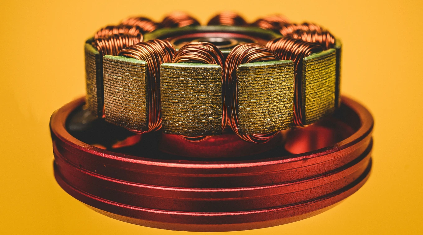
Before we begin analysing the BLDC motor, it's useful to be familiar with its different components and how they interact to make the motor spin. Here is a representation of a BLDC motor:

BLDC motors are cylindrical objects composed of two pieces:

• A stator: (static) depicted as the central part of the motor. It is composed of $s$ electrically controlled electromagnet called slots disposed radially. Slots are grouped in three phases depicted in ( ). Slots are connected by a core () usually made from a ferromagnetic material (Usually "laminated silicon steel to mitigate eddy currents").

• A rotor: (rotating) around the stator composed of $p$ permanent magnets called poles disposed with an alternation of north and south poles depicted in ( ) inside the edges of an enclosing ().

The functioning principle is simple: stator electromagnets exert a force on the permanent magnets of the rotor, driving the motor rotation.

To understand BLDC motors, a powerful tool to get familiar with is the magnetic circuit.

Magnetic circuit

Everything starts from Ampere's law for a static electric field in vacuum:

Ampere law

$$\nabla \times \B = \mu_0 \j$$

The curl ($\nabla \times \cdot$) of the magnetic field ($\B$) is equal to the permeability of the vacuum $\mu_0$ times the electric current density $\v{j}$.

However, things are a bit different in mater. To understand why, we need to differentiate between different "kinds" of currents:

• bound currents: tiny loops of currents inside atoms (denoted $\v{j_b}$)
• free currents: currents in conductors/charges moving through space at a "macroscopic level" (denoted $\v{j_f}$)

We can then split the magnetic field $\B$ into two fields $\M$ and $\H$ associated to the type of current and verifying:

• $\nabla \times \M = \v{j_b}$. $\M$ is called the magnetization field
• $\nabla \times \H = \v{j_f}$. $\H$ is called the magnetizing field

such that:

In some materials (ferromagnetic ones), the magnetization field depends on $\H$. In the absence of the $\H$ field, atomic magnetic dipoles are oriented randomly due to thermal agitation and cancel out at a macroscopic scale. However, when a sufficiently powerful field $\H$ is applied, they tend to align, creating a net magnetization $\M$.

We will suppose that this magnetization is proportional to the applied field $\H$ such that there exists a simple relation $\B = \mu\mu_0\H$ (i.e. $\M = (\mu - 1) \H \iff \H + \M = \mu \H$). Reality is more complex, but this approximation is sufficient for the scope of this article.

With this approximation we can write that in a linear, homogeneous material with constant $\mu$, combining $\nabla \times \H = \v{j_f}$ and $\B = \mu\mu_0\H$ we obtain locally:

Another very useful theorem in the context of electromagnetism is the Stokes theorem:

Stokes theorem

$$\iint_A \left(\nabla \times \B\right) \cdot \dA = \oint_{L} \B \cdot \dL$$

Where $A$ is an oriented surface with border $L$. $\dA$ is the vector orthogonal to the surface with magnitude equal to the area of the infinitesimal surface element $d\v{A}$. $d\v{L}$ is a vector tangent to the border $L$ of magnitude equal to the length of the infinitesimal border element $\dL$.

Combining it with our expression for the magnetic field inside a ferromagnetic material, we get that inside a ferromagnetic material we have for a current of intensity $I$ traversing the surface $A$:

i.e., the circulation of $\B$ on a closed loop $L$ is equal to the quantity of current $I$ that passes inside this loop multiplied by $\mu\mu_0$.

So if we take two loops of equal length, one which passes through a vacuum and one that passes through a ferromagnetic material with $\mu = 1000$, the circulation of $\B$ around the loop that passes through the ferromagnetic material will be $1000$ higher. In other terms, the magnetic flux tends to flow through ferromagnetic material.

As an example, if we consider a loop of length $L$ and cross-section $A$ made of ferromagnetic material with a copper coil wrapped around it $N$ times and traversed by an intensity $I$, we get the average circulation of the magnetic field lines loops inside the core (the ferromagnetic loop):

Finally, by introducing the following definitions:

• $\Phi \triangleq \iint_A \B \cdot \dA$ the magnetic flux through surface $A$
• $\mathcal{F} \triangleq NI$: the magnetomotive force
• $\mathcal{R}\triangleq L / (\mu\mu_0 A)$: the reluctance

We get:

This is Hopkinson's law:

Hopkinson's law:

$$\mathcal{F} = \mathcal{R} \Phi$$

This law can be thought of as a magnetic circuit analog of Ohm's law $U = RI$ for an electric circuit. In fact, we can push the analogy further using this table:

As for an electric circuit where current prefers the path of least resistance, enabling the confinement of current inside copper wires, magnetic flux prefers paths with low reluctance, enabling the confinement of magnetic field lines in ferromagnetic materials.

It is interesting to compare the ratio between the resistance of typical wires and the resistance of air with the ratio between the reluctance of typical silicon steel (a material commonly used for the core of electromagnets) and the reluctance of air. See link for the resistivity of copper and air and [link](https://en.wikipedia.org/wiki/Permeability_(electromagnetism) for the permeability of electrical steel and air

This means that magnetic circuits are more prone to leakage than electric circuits.

However, in this article, we will neglect leakage as an approximation and consider that all the flux created inside the core is exiting from the tip of the core.

Magnetic circuit components

We can describe different parts of a magnetic circuit by the relation between $\H$ and $\B$:

Air gap

In air, the magnetic field behaves as in free space, there are no bound currents, i.e., $\v{M} = 0$ and

Magnetic core

In a magnetic core, we have:

With $\mu \sim 1000$ a dimensionless constant called the relative permeability of the material.

Permanent magnet

A permanent magnet is like a ferromagnetic material where all the magnetic dipole moments are already aligned, thus the field $\H$ adds up to the magnetization $\M$, i.e.

Coil

A coil is exterior to the medium where field lines are, but as it is composed of free currents, it will influence the field $\v{H}$ through the relation:

We can obtain the integral version of this formula using Stokes' theorem along the magnetic circuit loop (do not confuse it with the coil loop, which is an electric circuit):

Thus

BLDC Magnetic circuit

We are now equipped to describe the magnetic circuit properties of a BLDC motor. A typical magnetic field line (depicted in ) will pass

• inside the coil through the magnetic core,
• through an air gap between the magnetic core and a magnet
• through a magnet
• through the rotor enclosing
• through another magnet
• through another airgap
• through another coil
• and finally get back to its starting point by passing through the core.

To simplify the math, we can analyze just half of this loop. We "cut" the loop at its axis of symmetry. By closing this path with virtual segments where the magnetic field $\H$ is zero or perpendicular to the path, we can apply Ampère's Law to a single "branch" of the motor.

For this unit circuit, the circulation of $\H$ is equal to the enclosed current $NI$ (the Ampere-turns of one slot):

Expanding this across the different materials (Magnet, Gap, Core, and the virtual segments where $\H$ is zero), we get:

Assuming $\B$ is uniform over the cross section of the circuit (i.e., $B = \Phi / A$), we can rewrite this in terms of the lengths ($l$) of each section:

And because $\mu \approx 1000$, $\mathcal{R}_\text{core} \ll \mathcal{R}_\text{gap}$ and $\mathcal{R}_\text{mag}$, we can approximate the reluctance of the magnetic circuit by:

Motor torque

Newton's law for rotating objects is:

With:

• $I$ the moment of inertia of the motor
• $\theta$ the angle of the rotor
• $\tau$ the torque applied on the rotor composed of
  • $\tau_M$ the torque resulting from the magnetic forces $\v{F_M}$
  • $\tau_L$ the torque corresponding to the load of the motor (e.g., the torque produced by the air opposing the rotation of the propeller)
• $b\dot{\theta}$ is the viscous forces with $b$ the viscous damping coefficient

We introduce some more notations about the geometry of the motor.

• $r$ is the radius of the motor (from the center of the motor to the center of the permanent magnets)
• $h$ is the height of the motor (height of the magnets)

By definition, the torque $\tau_M$ is

$\v{F_M}$ is given by the force applied by a magnetic field $\B$ on a magnet with a magnetic dipole moment $\v{m}$. It is:

In our case:

• The magnets on the rotor are pointing radially, and we will approximate them with an alternating magnetization $\M = \bar{M} \cos(\theta p / 2) \v{u_r}$ (something close to this can be obtained with appropriately shaped magnets) Note that the magnetization is the density of magnetic dipole moment $\M = d\v{m}/dV$.
• We will suppose that $\B$ is approximately uniform at the tip of the coil ($\B = \Phi / A \v{u_r}$)

For our magnetic circuit, the flux is given by Hopkinson's law:

Note that here, we don't include the magnet contribution to the magnetomotive force because we are interested in the force exerted by the coil on the magnet, (later when computing the back-EMF induced on the coil by the magnet, we will treat magnets as a source of magnetomotive force). Integrating over the surface of the gap and supposing that the magnetic field is uniform over this surface (e.g. $\B = \Phi / A_\text{gap} \v{u_r}$), we have:

(Note that $r$ vanishes at the third line because of the expression of the gradient in cylindrical coordinates)

Thus, the torque produced by one slot is:

And because a phase is composed of $s/3$ slots spaced by an angle $6\pi / s$, we can express the torque of one phase as:

Let's compute the sum:

Here we see that $1 - \exp(i\pi p) = 0$ because $p$ is even, thus we also need to have $1 - \exp\left(3\pi\frac{p}{s}\right) = 0$ for the torque to be not null, i.e.

Note that in real motors, the torque is not necessarily null when this condition is not satisfied. However, in general torque will be lower due to harmonic cancellation. If we now substitute $p$ at the third line, things simplify nicely, and we get:

Controlling the intensity as $I = \bar{I} \sin(\frac{p}{2}\theta)$ we have for one phase:

Combining the three phases using the following identity (with $\theta_e = \frac{p}{2}\theta$):

We finally get the total torque produced by the motor:

Thus, $n$ must not be a multiple of $3$ for the motor to produce torque. And in this case, the torque magnitude is:

It means that the torque $\tau_M$ is proportional to the intensity $\bar{I}$ we apply to the motor and also proportional to the radius $r$, height $h$ of the motor, the number of turns $N$ of the coil, the magnetization $\bar{M}$ of the permanent magnets and inversely proportional to one plus the ratio between the size of the air gap and magnet width. On a side note, the number of coil turns that one can pack scales linearly with the radius, such that, as a rule of thumb, the torque scales like $r^2 h$, the volume of the motor.

Motor power

Let's now analyse the power required to make the motor spin. As the rotor spins, the magnetic field oscillates. It creates an electric field $\v{E}$ that will generate an electromotive force (back-EMF) in the winding. This force will act as a power supply of voltage $V_\text{EMF}$ (it is the same principle as a dynamo). The Maxwell-Faraday law tells us the strength of the back-EMF:

Maxwell-Faraday

$$\nabla \times \E = \partial_t \B$$

From which we can derive the Faraday's law of induction

Faraday's law of induction

$$\begin{align*} V_\text{EMF} &=-\frac{d\Phi}{dt} \end{align*}$$

The flux $\Phi$ is computed using the same magnetic circuit approach as before, but using the permanent magnets as the source of the magnetomotive force instead of the coils. The magnetization can be seen as a measure of the quantity of current loops that a line is traversing when passing through it. It is expressed in ampere per meter. The magnetomotive force associated with a field line is thus:

And In our case with magnetization $\M = \bar{M} \cos(\theta p / 2) \v{u_r}$ over a surface spanning an angle $2\pi/s$ and height $h$ at a distance $r$ from the center, integrating over the magnet width $w$ we get:

The reluctance of the magnetic circuit is the same as before, thus for one turn of the coil we have:

And accounting for the $N$ turns of the coil, we get:

To get the power drawn by the first phase, we multiply by the intensity $I = \bar{I} \sin(\frac{p}{2}\theta)$.

Combining the three phases with the same identity that we used when computing the torque, the $2/3$ factor cancels, and we finally get:

First, we can notice that $K_V = K_\tau$. This is expected as $P_\text{electrical} = P_\text{mechanical}$ because of energy conservation. And indeed, we have:

Thus, $K_V = K_\tau$; we could have deduced it right after determining $K_\tau$, but it's always better to check that everything is consistent.

Other sources of voltage include the resistance $R^\phi$ and inductance $L^\phi$ of each phase for a total voltage experienced by the winding of:

Let's compute the contribution of the resistance and inductance for one phase:

Combining the three phases with the same identity as before, and noticing that in addition to the identity, we also have:

We finally get the total power consumption of the motor:

The resistance of a single phase (composed of $s/3$ slots) is simply the resistance of the copper coils, which I give the expression here:

Trying to estimate $L_\text{turn}$ and $A_\text{wire}$ can be tricky. So I will not give an estimation formula. But you can notice that $A_\text{wire}$ will scale like $\frac{r^2}{sN}$ and $L_\text{turn}$ will scale like $h + Cr$ with $C$ a constant thus the resistance roughly verify:

Thus, the efficiency of the motor is:

Reality check

To calculate the gap between theory and reality, let's use the T-Motor Antigravity 4004 (KV300) as our benchmark.

Based on the data sheet/pictures/drawings, and common material properties:

• Geometry: $r\approx20\text{ mm}$ ($0.02 \text{ m}$), $h=7 \text{ mm}$ ($0.007\text{ m}$).
• Magnets: Neodymium (sintered), so $\bar{M} = 9.5\times 10^5 \text{ A}\text{ m}^{-1}$. (since $B_r \approx 1.2 \text{ T}$ and $B_r = \mu_0 \bar{M}$)
• Windings: Let's estimate $N=25$ turns per slot (counting on the picture they say single wire thick but it seems to have two layers).
• Configuration: $s=18$, $p=24$ (counting on the pictures).
• Air gap/Magnet ratio: $1$ (from the pictures the air gap is about the same size as the magnet thickness).
• Resistance: $R = 452\text{ m}\Omega$ (from the data sheet)

Using our formula for $K_\tau$ we have:

Substituting the values:

Now, let's convert $K_V$ to (RPM/V). In SI units, (rad/s per Volt). To get the hobbyist unit (RPM/V) (remember that $1 \text{ V} = 1 \text{ N} \text{ m} \text{ s}^{-1} \text{ A}^{-1}$):

A 2-3% error is actually good for a first-principles derivation! I probably got lucky with the parameters I chose, but it shows that the model is capturing the essential physics of the motor. In reality, there are many other factors that can affect the performance of the motor, such as:

• Non sinusoidal magnetization and current waveforms
• Magnetic saturation of the core
• Magnetic leakage
• Non-uniformity of the magnetic field
• Eddy currents and other losses
• Manufacturing imperfections
• Temperature effects on the resistance and magnetization

Conclusion

In this article, we have derived from first principles the magnetic circuit properties of a BLDC motor and used them to compute the torque and power of the motor. We have also compared our theoretical predictions with the specifications of a real motor and found a good agreement. I really enjoyed writting this article, it was a great opportunity to apply the concepts of electromagnetism that I learned in school to a real-world application. I hope you enjoyed reading it as much as I enjoyed writing it! If you have any questions or suggestions for improvement, please feel free to reach out to me.